Introduction To Cartesian Plane

$\underline{I.\ Defining\ A\ Cartesian\ Plane}$

The Cartesian plane is a plane formed by two number lines intersecting each other at $90^\circ$.

Below is the diagram of a graph sheet, with the minor gridlines removed for clarity.

We have drawn the two axes in blue color, with arrow at the two ends of each line. The horizontal axis called the $X$ axis and the vertical axis is called the $Y$ axis. Each of these axes is a number line, and the intersection point is called the $origin$ and it has a value of $0,\ 0$.

-----------book page break-----------

Let us first understand the terms that we will be coming across in our subsequent readings or problems.

$\underline{Point}$

Any random point selected on the graph sheet has a unique $X$ and $Y$ value, written as $(X,\ Y)$. These values are called the co-ordinates of the selected point. We will see examples below.

$\underline{X\ axis}$

The axis along which we will measure the $X$ value of any point. In the above diagram this is shown as a horizontal line in thick blue.

$\underline{Y\ axis}$

The axis along which we measure the $Y$ value of any point. In the above diagram this is shown as the vertical line in thick blue.

$\underline{Major\ gridlines}$

The lines drawn above with green, parallel to the two axes, are called major gridlines.

$\underline{Minor\ gridlines}$

The thinner lines in between two major gridlines shown below are called the minor gridlines.

$\underline{Origin}$

The origin is the point whose $X$ and $Y$ values are $0, 0$

-----------book page break-----------

$\underline{II.\ Scale}$

This is the measurement scale across both axis. In the graph above we have taken a scale of $one\ major\ division = 5$.

You can choose your own scale that suits the value ranges that you are handling.

Now we will see how to plot points on the graph sheet. Take a look at the graph sheet below.

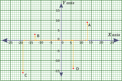
First of all let's see what scale we chose for the graph. We selected each large division (distance between to major gridlines) as $5$. That also means that each small division (distance between two minor gridlines) is $1$.

-----------book page break-----------

There are four points, named $A$, $B$, $C$ and $D$ on the graph sheet, each marked with a red dot.

We will try to reach each of the points, every time starting from the origin.

How do we reach point $A$ from the origin, using the shortest path, moving only in horizontal or vertical directions?

To reach point $A$ we can move $13$ units to the right (in the positive $X$ direction) and $9$ units up (in the positive $Y$ direction). This is the shortest possible path. Since we more $13$ units in the positive $X$ direction and $9$ units in the positive $Y$ direction, the co-ordinate of point $A$ is $(13,\ 9)$.

Similarly, to reach point $B$ from the origin, given the conditions above, we need to move $13$ units to the left (the negative $X$ direction) and $3$ units up (in the positive $Y$ direction).

Therefore, the co-ordinate of point $B$ is $(-13,\ 3)$.

Same way, if you follow the arrows shown in the diagram, you will see that the co-ordinates of point $C$ is $(-19,\ -21)$ and the co-ordinates of point $D$ is $(6,\ -14)$.

Now we will look at one more definition.

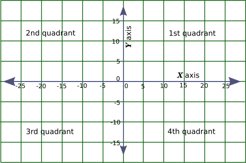
$\underline{III.\ Quadrant}$

The $X$ and $Y$ axes, as shown in the diagrams above can be extended indefinitely to cover the entire graph sheet. Once we do that we can see that the graph sheet is divided in four regions, one to the top-right of the origin, one to the top-left of the origin, one to the bottom-left of the origin and the last one to the bottom-right. Each of these regions is called a $Quadrant$.

-----------book page break-----------

The properties of these quadrants are as follows:

$\underline{1\raise{3px}{st}\ Quadrant}$

This is the region above the $X$ axis and to the right of the $Y$ axis.

All points in this region have a positive $X$ value and a positive $Y$ value.

$\underline{2\raise{3px}{nd}\ Quadrant}$

This is the region above the $X$ axis and to the left of the $Y$ axis.

All points in this region have a negative $X$ value and a positive $Y$ value.

$\underline{3\raise{3px}{rd}\ Quadrant}$

This is the region below the $X$ axis and to the left of the $Y$ axis.

All points in this region have a negative $X$ value and a negative $Y$ value.

$\underline{4\raise{3px}{th}\ Quadrant}$

This is the region below the $X$ axis and to the right of the $Y$ axis.

All points in this region have a positive $X$ value and a negative $Y$ value.